Transformations Benchmark

Random Graphs Generation

To evaluate rsppfp package, several examples were benchmarked. This is run using 27 randomly generated graphs, which result from the combination of the following values:

• A set of nodes of sizes: size(N) = {100, 300, 500}
• The number of forbidden paths varying according to size(F) = {50, 250, 500}
• A varying densite of size(d) = {0.1, 0.5, 0.9}

A total of 27 graphs were generated using igraph’s erdos.renyi.game(...), and the forbidden paths were constructed with their random_walk(…) function; results were limited to prevent walks of less than three nodes.

# Checks if the path is part of any row of the forbidden subpaths.
# Returns the logical comparison of the evaluation.
already_exists <- function(fp, path) {
  return( any( 
    apply(fp, 1, function(x) str_detect(paste(x, collapse=","), paste(path, collapse=","))) 
  ))
}


# Checks if a forbidden paths contains a subpath of another forbidden path.
# Returns the logical result of the comparison.
has_subpath <- function(fp, path) {
  # If the length if 3, evaluate as-is
  if(length(path) == 3) {
    return(already_exists(fp, path))
  }
  # Otherwise
  else {
    # We need to generate subpaths of length three
    for(i in 1:(length(path) - 2)) {
      # Check if the value is a subpath. If it is, return immediately
      if( already_exists(fp, path[i:(i+2)]) ) return(TRUE)
    }
    
    # If we got here, return false
    return(FALSE)
  }
}


# Creates random graphs using a specific seed.
# seed <- 1111
get_random_graphs <- function(seed, directory) {
  # Set a random seed
  set.seed(seed)
  
  # Prepare values
  nodesNumbers <- c(100, 300, 500)
  densities <- c(0.1, 0.5, 0.9)
  fpathsNumber <- c(50, 250, 500)
  
  
  # Create the dataframe
  graphsInfo <- data.frame(
    nCount = numeric(),
    nCountReal = numeric(),
    aCount = numeric(),
    density = numeric(),
    fCountTheoric = numeric(),
    fCountReal = numeric(), 
    gfile = character(),
    fFile = character(),
    stringsAsFactors = FALSE
  )
  
  
  # Loop through the node count
  for(nodeCount in nodesNumbers) {
    
    # Loop through the density
    for(d in densities) {
      # Get the arc count
      arcsNumber <- (nodeCount ^ 2) * d
      
      # Create a graph
      graphI <- erdos.renyi.game(nodeCount, arcsNumber, directed = TRUE, type = "gnm")
      
      # Remove nodes without edges
      graphI <- delete_vertices(graphI, V(graphI)[ degree(graphI, v = V(graphI), mode = "total") == 0])
      giDF <- as.data.frame(get.edgelist(graphI)) %>% `colnames<-`(c("from", "to"))
      
      # Loop on the number of forbidden paths
      for(fpCount in fpathsNumber) {
        
        # Get the starting nodes for forbidden paths
        randomStartNodes <- sample(x = V(graphI), size = fpCount, replace = TRUE)
        fpDF <- data.frame(matrix(ncol = 6, nrow = 0))
        
        # For each element there
        for(rsn in randomStartNodes) {
          
          # Get a random number of steps
          rSteps <- sample(3:6,1)
          
          # Create a random walk through the graph
          rWalk <- random_walk(graph = graphI, start = rsn, steps = rSteps, 
                               mode = "out", stuck = "return") %>% as.vector()
          
          # If it is at least 3 nodes long and has no subpaths
          if(length(rWalk) >= 3 & !has_subpath(fpDF, rWalk) ) {
            # Then add it to the list
            fpDF[nrow(fpDF) + 1, ] <- structure("length<-"(rWalk, 6), class = class(rWalk)) 
          }
        }
        
        # Record the files
        gFileName <- paste0(directory, "/", nodeCount, "Graph_", (d * 100), "pDense_", fpCount, "fp_Graph.csv", 
                            collapse = "")
        fFileName <- paste0(directory, "/", nodeCount, "Graph_", (d * 100), "pDense_", fpCount, "fp_Paths.csv", 
                            collapse = "")
        write.csv(file = gFileName, x = giDF, row.names = FALSE)
        write.table(fpDF, fFileName, na = "", row.names = FALSE, col.names = FALSE, append = TRUE, sep = ",")
        
        # Append to the dataframe
        graphsInfo[nrow(graphsInfo) + 1, ] <- 
          list(nodeCount, length(V(graphI)), arcsNumber, d, fpCount, nrow(fpDF), gFileName, fFileName)
      }
    } # End densities loop
  } # End arc count loop

  
  # Return the values
  return(graphsInfo)
}

Benchmark Results

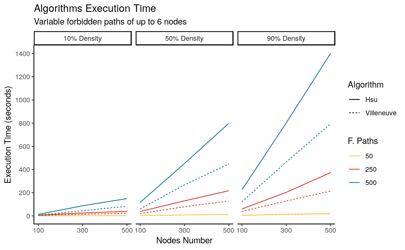
Figure 1 shows the results for digraphs of each density. This was executed on a computer with an Intel I7-4790 CPU at 3.6Ghz, with 4GB of RAM, using Linux Ubuntu 16.04 as the operating system. Three cores out of four were used in all of the transformations.

As can be seen, in all situations the more general algorithm (Hsu’s) takes longer to complete, though this difference increases with the number of forbidden paths and density. It is worth mentioning that this is expected behavior, as the transformation logic iterates on the forbidden paths F –each one needs to be individually evaluated to add new nodes and arcs to the graph. Because of its logic, Hsu’s backward construction always produces a smaller gStar with less nodes and arcs, while Villeneuve’s algorithm is slightly faster; this difference is noticeable for larger values of F.